Fixing wild Spinning in Tachyon: The fringe

Dilli, I’d like to get off Mr. Bones wild ride

- Jake Logan, probably

Glide wrappers can be both a savior and a menace sometimes. The game looks great with them:

 But on every start of a new level you get uncontrollable spinning of your ship. The spinning looks to be always on a \ diagonal - so what's going on? Can we fix that? Let's open the game up in ghidra and see what we can figure out. The issue must come from some faulty cursor logic, right? My initial gut reaction was to trace DxInput:

 

The game for some reason sets up two dxinput interfaces. I looked around the two caller functions and it seems the second one is specifically for joystick input, while the first one enumerates devices and sets callbacks. That didn't help me either way. Ok, what about functions that deal with the cursor? Are there any? 

 

Bingo!  That ClipCursor and SetCursorPos are readily good contenders for where bugs around spinning ship might happen. ClipCursor restricts cursor movement to a rectangle, and SetCursorPos moves the cursor where the game wants it to be.

 

 

By the time I took the screenshots, I already went and explored some of the functions that call these functions - that's why They have reasonable names. You'll see nothing but FUN_XXXXXX if you just opened space.exe for the first time in ghidra. But those functions are decently small and don't refer to many static variables, which should be somewhat straightforward to figure out what they do. To be honest, I still don't fully understand this system. It appears all of UI is hard-coded to be at 640x480, including mouse pointer lock. Then during the game, window sizes are taken into account and numbers are adjusted accordingly. 

If you trace those ClipCursorToX and ExpandCursorPosition functions you'll find that They are used in the main window process function:

Quick shout out to pinvoke.net - that's the cleanest source of Windows' constants I was able to find. We see that when the message is 0x1c - it's WM_ACTIVATEAPP message. And reading the documentation for WM_ACTIVATEAPP we see that when wParam is false, the window is being deactivated, when it's true - activated. There's a layer of indirection here - I guess the code was meant to substitute different activation/deactivation handlers, but lukcly current addresses in the binary point to exact functions used

 

And it just so happens that these are the functions that call our ClipCursor eventually:
 

Ok, so for those who are more familiar with the bug - the bug gets cleared when we alt-tab from the game and go back in - to it's these two functions - onWindowActivate at address 0x432d80 and onWindowDeactivate at address 0x432dc0 that end up "fixing" the bug. 

I spent some more time looking at the SetCursorPos function and who calls it. This allowed me to uncover the static structure in the game that relates to all things mouse:

 

 

I use my own little convention of adding _maybe to functions or data that I'm not certain used exactly so. You'll also notice a lot of green labels from Ghidra - that's an indication of static data.  E.g. CONFIG_CURSOR.pos.x is at 0x603e40 and y is at 0x603e44 - you should be able to add these addresses in something like Cheat Engine to see the mouse coordinates the game using right now.

From there I was able to find this really interesting function - and that's how the game actually gets mouse position data to begin with:

 

Only one function ever calls this PeekMouseMessages, and only one more function calls it. I spent some time exploring those functions. It's good to trace not only up and down the stack but also to look how some data gets moved around and what writes to this data. By a total accident from a different effort I ended up finding how the game reads config files and stores their data in memory. From there I've already touched this value before:

 

What is this MOUSE_NO_TOGGLE?  The game reads it from a config file and if I grep -irn NO_TOGGLE inside of the game directory I get a single hit to the readme: 

======================================================================
6. Corrections to the Manual:
======================================================================
* Mouse Controls: The mouse controls have been enhanced for
easier use. The mouse defaults to Fine Look controls (formerly
you had to hold down right mouse button for this mode).  Pressing
the right mouse button now toggles between Fine Control and Fast
Turning Control. You do not have to hold down the right mouse
button anymore to stay in either mode. If you prefer the style
detailed in the manual and keychart, simply open up the
Tachyon.cfg file with WordPad. Under the [CONTROL] section,
change MOUSE_NO_TOGGLE=0 to MOUSE_NO_TOGGLE=1, then save the
file.  

So the function that calls our PeekMouseMessages() is actually Mouse_FineMoveControls()! And it looks like this once you rename some statics:

 

More over the sole caller is:

So at this point I sat there for a while looking for bugs in any of these functions. There's some edge-case between how the game clips the cursor and gets the mouse coordinates that makes the ship spin uncontrollably... but only with a glide wrapper, and only with some of them... I don't know all things glide wrappers do and I didn't want to spend time understanding them either... But I did remember how alt-tabbing fixes the issue... And everything works fine in the menus - only after level load something messed up happens. Perhaps that's when screen resolution changes? What if we just force the game to recalculate clip region after a level loads? Luckily, from a previous effort I've already identified function that switches from loading screen to playing the game:

 

This is a function located at 0x44ec80 in Steam version of the game. All we need to do is call a function that re-calculates cursor clipping coordinates between showing the loading screen and playing a level... And luckily we already have a function that does that - onWindowActivate. I've patched a jump to some unused executable memory first after the return of the loading screen call and added a call to onWindowActivate there. And suddenly there was no more spinning!

Reverse Engineering Video Game Assets: Part II

 Now that we figured out main asset storage in Part I, we are ready to start figuring out how to get more out of the extracted files. I used the extractor and saved each individual file - there are 8132 files there. Running  ls | cut -d'.' -f2 | sort -u  gives us the following list: anm, bas, bdf, bin, bmp, box, cfg, def, des, hud, ion, itm, job, mnu, mp3, mpc, nws, ocf, pak, pal, pcx, pix, psd, pwf, scr, sen, spx, txt, vcs, wav, wng. These are all of the different file extensions. We can run GNU's file command on those to figure out what is a known file type and what isn't:

$ for ext in $(ls | cut -d'.' -f2 | sort -u); do ls *.$ext | head -n1 | xargs file; done

gate_flr.anm: data

bdispute.bas: data

bora1.bdf: data

base0.bin: data

skin.bmp: PC bitmap, Windows 3.x format, 128 x 128 x 8, image size 16384, resolution 2834 x 2834 px/m, cbSize 17462, bits offset 1078

borders2.box: data

cargo.cfg: data

face.def: data

aclrng.des: data

archangl.hud: data

descript.ion: data

ammohold.itm: data

bora00.job: data

bora.mnu: data

agtb010.mp3: MPEG ADTS, layer III, v1, 48 kbps, 44.1 kHz, Monaural

basewar1.mpc: ASCII text, with CRLF line terminators

bora20.nws: data

arena.ocf: data

aarm2.pak: data

aarm2.pal: PCX ver. 3.0 image data bounding box [0, 0] - [15, 15], 8-bit colour, RLE compressed

a_agt.pcx: PCX ver. 3.0 image data bounding box [0, 0] - [255, 255], 8-bit colour, 72 x 72 dpi, RLE compressed

preview.pix: Apple HFS/HFS+ resource fork, map offset 0x2126, map length 0x3f, data length 0x2026, list offset 0x1c, name offset 0x32, 1 type, 0x50494354 'PICT' * 1 resource offset 0xa

nws_brix.psd: Adobe Photoshop Image, 256 x 256, RGB, 3x 8-bit channels

menus.pwf: data

2mrch.scr: data

b3bc040a.sen: data

bora01a.spx: data

tachycre.txt: data

vcs.vcs: ASCII text, with CRLF line terminators

1gplt01.wav: RIFF (little-endian) data, WAVE audio, IMA ADPCM, mono 22050 Hz

global00.wng: data

 The command just takes the first file with such extension. I'm assuming all files with the same extension can be parsed with the same parser here (I later found that's not true in all cases in this game). I was quite surprised to see apple resource fork and a photoshop image in the dump. I quickly scanned the fork with hexdump and it appears to contain extra data about the photoshop image, so maybe someone copied something on accident into the archive? In either case it's fun exploring the pcx images and mp3/wav sounds. Lots of nostalgia for me; but that's not why we're here. The game is 3D... where are those 3D models? 

I've spent some more time looking at Tachyon.exe - the parent function that opens the pff file reads the name of this file from another file kind that's called "RTXT" in the binary. After spending some time defining structures and renaming functions - I had a complete view of the RTXT file format. More over there was a very similar file format called "CBIN" - they are essentially ini files - have sections, keys and values. Except all strings are interned, and values can be a string, a float, or an int - and the binary version of the value is stored (as opposed to string). 

#[derive(BinRead, Debug)]

struct RTXTHeader {

magic:[u8;4],

section_info_offset:u32,

_unk:u32,

entry_count: u32,

}

#[derive(BinRead, Debug)]

struct ResourceEntry {

string_offset: u32,

_unk1: u32,

_unk2: u32,

_unk3: u32,

}

#[derive(BinRead, Debug)]

struct SectionEntry {

first_key_offset: u32,

keys_in_this_section: u32,

}

 

#[derive(BinRead, Debug)]

struct CBINHeader {

magic:[u8;4],

config_bytes:u32,

string_bytes:u32,

string_entry_count: u32,

decryption_key: u32,

}

#[derive(BinRead, Debug)]

struct CBINHeaderDecrypted {

magic:[u8;4],

config_bytes:u32,

string_bytes:u32,

string_entry_count: u32,

decryption_key: u32,

section_count: u32,

}

#[derive(BinRead, Debug)]

struct LabelledEntry {

label_index: u32,

entry_count: u32,

}

 

Both follow approximately the same file structure, except CBIN is encrypted and uses the same decryption method discussed in part one. As you see the unknown fields are present - the code doesn't seem to touch them, but they are needed fro proper offset computation. Once you can parse those files you'll see that these two compose majority of the file in the game archive - bas, bdf, cfg, bas, des, job, mnu, nws, itm - are all either CBIN or RTXT files which again makes them essentially packed ini files, that can be loaded directly into memory without really much parsing - the format is definitely optimized for speed - and it shows - the game code actually just loads files into ram, quickly replaces any _offset fields to be actual pointer, and that's it.... Then the game uses the structs I showed above during all kinds of game logic to read game state or config - like how many credits you have.
After filtering out all the files that are CBIN or RTXT (side note - I should learn how to teach GNU file application to recognize new formats) we are left with *.pak, *.pwf, *.scr, and *.spx files. This is where some knowledge of the game itself can help, or you can explore those countless config files - the starting ship is called Orion. And there just so happens to be only orion.pak out of the extensions we can't read yet. More over orion.des is actually a config file which tells you info about orion as a game-object, and has a "PAK=orion.pak" config line.  Ok so we need to figure out how to read pak files. Well it's time to open up space.exe in ghidra... WTF?

The entry point is giant 978 lines of decompiled C-code function that does oh so many function calls, XOR data decryptions, and random checks. That's not natural! Ghidra analysis also was not able to find too many other functions. So the binary is encrypted/obfuscated. My first reaction was to try and reverse engineer the obfuscator. I found some XOR keys and went looking at the data I could decrypt - it wasn't much help though as it seems the obfuscator would stage some code on the stack, execute it, then repeat the process several times. This is actually where my other problem lived - modern Linux, wine, Windows (and Macos for that matter) do not allow for executable stack. A while ago we figured out that that was just an open invitation to viruses, so operating systems quickly implemented "non-executable stack". But now wine can't run the game because as soon as the game tries to decrypt itself on the stack wine detects call to stack and crashes the game, thinking it's a virus. Proton, however seems to have that case handled correctly. (Side note, I've heard GoG version runs on wine natively. I don't know if they have a different version of the obfuscated code or what). 

Well, I know proton runs the game correctly... let's see what the code looks like when the game is passed the obfuscator entry. At this point you need to know the difference between a program stored in an executable file versus running in memory. 

 

All operating systems have a "loader" module, which takes an executable file stored on your drive, and load it into memory. The file on disk consists of several sections - .text, where the machine code of the program is stored, .rdata - where read-only data is stored. .data - where initial values of dynamic data are stored. There are plenty of other sections possible, but those are the ones we are interested the most. What happens is that the loader, loads sections into memory, maps the addresses correctly, and tells the CPU to start execution of whatever is the entry point. In our case the entry point is our large obfuscator. So there's a good chance the obfuscator does something and that something results in an actual game code being stored somewhere and executed. So once the game enters the main menu, at least some code needs to be deobfuscated. Later I learn that it deobfuscates just the whole game at a time and conveniently writes it all back into .text section in memory. That section just never gets stored back to the drive... We can fix that. 

I'm not certain how to do this on Windows, but on Linux there are several ways to store all of the program's running memory to disk - it's called a core dump, and one of the ways to do it is to call $ gcore <pid> . You can find the pid by running ps aux | grep space.exe . This will cause approximately 2GB file to be created. Lots of tools can open core dumps. Since we're already using ghidra we can open the core dump in it! Watch out though - when ghidra asks to analyze the file - DON'T DO IT! It'll take more than an hour. At this point I also want to mention a challenge - I'm running a 64-bit linux, which uses wine to load a 32-bit windows game. This confuses ghidra because it assumes a single file is meant for a single target platform. Luckly this doesn't affect us - I looked at the core dump's .text section and manually compared its random offset with data in space.exe - and it was different! So I extracted this data into a separate file, then opened original space.exe and replaced its .text with the newly extracted one... Voila! 

We know it worked because we were able to re-analize the file and find a LOT more functions. What's even better is that we were able to find a lot of imported functions. This is where knowing basics of windows development can help - to create a window someone needs to call the CreateWindow* function:

 

 This function has only one reference:

I've spent some time recovering UI context - you'll see a lot of DAT_ values instead. Let's go back to looking for info about our pak files! To make life a bit easier I also loaded the .rdata and .data sections from our core dump - the more the merrier in this context:

If you see some of the UPPER_CASE strings and search for those strings in the extracted game files you'll find that *.des files have EXTERIOR_PAK key that points to ship's pak.While good approach in general - in our case there's a lot of references to this string:

 

We can also look for more strings, or do the trick with fopen. There's a lot of "try different strategies" here. What I did was I went to look for strings that I was already familiar with from the game launcher - Tachyon.exe. Since the game reads the same resource file - there's a good chance that the exact same functions are in it. I ended up finding this function - file_OpenEx (I know its name because it logs its name on error). From there I went back up the XREFs of file_OpenEx and marked every argument that is a filename passed to file_OpenEx. It so happens that FUN_004b14b0 calls file_OpenEx, and at some point gets called with "moveroid.pak" filename. So it's a good chance that's our PAK parser! We are going to go over it in Part III.

Reverse engineering video game assets: Part I

Long time ago when I was a kid I used to play this video game that I really like... I'm not going to name it because I'm not sure if anyone still cares for this game, but it was released in 2000 for Windows 98 and I think there were rumors for a PlayStation1 release, but that never happened. The game is currently sold on GoG, Steam, and probably a few other platforms. It runs on Windows and Linux thanks to Steam's Proton. Though I hear GoG version runs on plain Wine as well. 

Well damn it, I was not satisfied that I couldn't run this 25 year old game at my 4K resolution and 144Hz. So like any self-respecting masochistic ignorant nerd I said "Sure, I can remake this in Rust". This is how my journey stared. According to Ghidra, the game is ~260K source lines of code when decompiled. I'm not "dreaming" to remake this game in Rust, but loading all of the assets in Bevy actually helped the reverse engineering efforts, so so far that's where I'm heading. Information in this blog post isn't new (shoutout to FringeSpace folks for advising and moral support). However a lot of the reverse engineering efforts have been ad-hoc and it sounds like on average I have already caught-up with what has been recovered in the past 25 years. I wanted to attract/teach people reverse engineering games for modding/preservation and also a single-place repository for information about this specific game's file structures, so that's why I'm making these blog post series.

You don't need to know reverse engineering, ASM, ghidra, or imhex to enjoy this blog post, but you need to know your C.

So let's dive right into it. This post's goal is to figure out how the game stores its asssets, whatever those are. I downloaded the game through Steam and look at the files:

 

The command just sorts files by size and removes dlls from view. The big outlier is Tachyon.pff taking the majority of the folder's size - 365MB. That's likely our target. I tried running common file ID tools against it and searching online, and while I did find the FringeSpace community who already RE'd the file - the consensus was that the PFF file structure was internal to the company that developed this game. So What can we do? Well the game reads the file... so it should have code inside of it that reads the file... let's open it in ghidra and see what happens. 

 

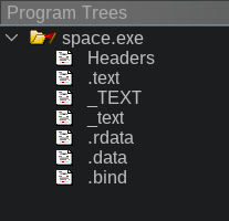
 I should note that I made a mistake already - Tachyon.exe is a small intro app that lets you browse the authors' website, look for updates, and configure the game before running it. This isn't the actual game, which is the 1.8MB space.exe executable that you see in the file listing above. However this mistake was fruitful at the end - the main game binary is obfuscated while this intro app isn't. At the same time - both the intro app and the main game load Tachyon.pff file - so we're in luck!

 

When you open Tachyon.pff in Ghidra it presents you with this view. I'd like to note that my view isn't quite default - I adjusted the color theme and added a few windows I find useful at the bottom. All of these can be added from the Window pulldown menu. Quick note about Jython - it's python with ghidra's java bindings. It can be useful for quick scripting, but I find the console presence to be really nice for quick dec->hex->bin conversion.

So at this point there are several things we can do. Before I dive into what I did - let's think for a second what is Reverse Engineering? I like to think of RE as pumping context into math, and you are the pump. Context being this abstract multidimensional latent space that you know. Ok so what do you know about this game? What do I know about it? Well, I know I want to find how to read tachyon.pff file. So I can search for strings and see if one of them is tachyon.pff. I also know that the only way to open files is to ask Windows to open them for you - so we can look for variations of the open() function.

 

When searching for strings - I was not able to find the whole word - tachyon.pff in the file. Bummer. But I was able to find these really interesting strings - this has to be used somewhere where I need to look, right?

If we click on one of the strings - the listing view will take us to it. From there we can see that Ghidra found exactly one function that references this address (the XREF label) - click on that function and you'll see: 

byte * FUN_0040b0a0(uint *param_1,undefined4 *param_2)

{

bool bVar1;

undefined3 extraout_var;

byte *pbVar2;

UINT UVar3;

bVar1 = FUN_0040aec0(param_1,param_2);

if (CONCAT31(extraout_var,bVar1) == 0) {

param_2[0x2d] = 1;

pbVar2 = NULL;

}

else {

UVar3 = FUN_0040afb0(0,2,param_2);

FUN_0040afb0(0,0,param_2);

param_2[0x2c] = UVar3;

DAT_0047fb44 = UVar3;

pbVar2 = (byte *)FUN_004063a0(UVar3,4,0,0x42e578);

FUN_0040af60(pbVar2,UVar3,param_2);

if ((*(uint *)param_2[0x27] & 1) != 0) {

FUN_0040b060(pbVar2,UVar3);

}

param_2[0x2d] = 0;

}

return pbVar2;

}

 Ok, where is that string?

Unfortunately the analysis didn't propagate the fact that this data is a human-readable text to the decompiler. Let's look back to where the string is stored - it's at 0x42e578... Oh look the code lists that as a fourth argument to this other function call - FUN_004063a0. We can right click on it and change parameter definitions:

 

Ok, so looking at the code now, we call FUN_0040aec0, then if that variable is 0, we return null, otherwise we do something and call a function that says "PFF LOADED FILE" ok, that sounds like we're in the right place. 

Remember how I mentioned that reverse engineering is pumping context into math? Well, we are looking at some function and we just got a bit of context - it loads a pff file successfully. Now we need to nudge context from random directions until we bring enough of it to figure out what this function does. I like strings. Human readable strings is where a lot of context lives for us. During my first run-in with this file I went the manual way. I looked at this function, looked at other functions nearby, looped for KERNEL32.DLL::_lopen() function and see who called that... Eventually I brought enough context to figure this function out. However I also developed a few scripts to help me along the way. One of them is modification of ghidra's standard recursive string finder, however I modified it slightly - It now prints not only strings, but function names and static label names that don't start with FUN_ or DAT_ or LAB_ - essentially everything that I manually named already. Let's run that script on this function:

CALL FUN_0040b0a0 ()

@0040b12d - CALL FUN_0040af60 ()

@0040af7c - CALL FUN_00407210 ()

@00407228 - SYMBOL: PTR__lread_0042e0b8

@0040b109 - SYMBOL: s_PFF_LOADED_FILE_0042e578

@0040b116 - CALL FUN_004063a0 ()

@004063c1 - ds "mem_GetMemEx(): %ld bytes ('%s')\n"

@00406501 - SYMBOL: s_mem_GetMemEx():_Failed_to_alloca_0042e3ac

@00406501 - ds "mem_GetMemEx(): Failed to allocate %ld bytes ('%s')"

@004063de - SYMBOL: PTR_DAT_00430f54

@004063cb - CALL FUN_0040fc1a ()

@0040fc43 - CALL FUN_00411a1e ()

@00411dc8 - SYMBOL: PTR_FUN_00431380

@00411fe2 - CALL __aulldiv ()

@00411e87 - SYMBOL: s_null)_0042e78d

@00411e00 - SYMBOL: PTR_FUN_00431384

@00411e1e - CALL _strlen ()

@00412078 - CALL FUN_00412194 ()

@004121ae - CALL FUN_0041215f ()

@0041217c - CALL FUN_00411909 ()

@00411975 - CALL FUN_004153c8 ()

@004153d3 - CALL _malloc ()

@0041199e - CALL FUN_00414b2f ()

@00414c54 - SYMBOL: PTR_GetLastError_0042e0e0

@00414b88 - CALL FUN_00414a95 ()

@00414af1 - SYMBOL: PTR_GetLastError_0042e0e0

@00414ae4 - SYMBOL: PTR_SetFilePointer_0042e0a8

@00414c07 - SYMBOL: PTR_WriteFile_0042e168

@00411c77 - SYMBOL: PTR_DAT_0043139c

@00411a8c - SYMBOL: switchdataD_0041213f

@00411cf2 - CALL FUN_004154eb ()

@00415534 - SYMBOL: PTR_WideCharToMultiByte_0042e14c

@00411c94 - SYMBOL: u_null)_0042e77e

@00411bbd - SYMBOL: PTR_DAT_00431150

@00411e87 - ds "null)"

@00411de9 - SYMBOL: PTR_FUN_0043138c

@00411d82 - SYMBOL: PTR_DAT_00431398

@00411fd0 - CALL __aullrem ()

@004063d8 - SYMBOL: PTR_OutputDebugStringA_0042e0cc

@004063c1 - SYMBOL: s_mem_GetMemEx():_%ld_bytes_('%s')_0042e3e0

@0040b0b1 - CALL FUN_0040aec0 ()

@0040aed1 - CALL FUN_0040ade0 ()

@0040ae09 - CALL FUN_00416a2c ()

@00416a73 - CALL FUN_004122fc ()

@0041230b - SYMBOL: ExceptionList

@0041235a - SYMBOL: PTR_LCMapStringA_0042e140

@0041233e - SYMBOL: PTR_LCMapStringW_0042e13c

@004123db - SYMBOL: PTR_MultiByteToWideChar_0042e144

@00412509 - SYMBOL: PTR_WideCharToMultiByte_0042e14c

@00416abc - CALL FUN_0040fe1b ()

@0040fe42 - SYMBOL: PTR_HeapFree_0042e174

@0040fe31 - CALL FUN_004130a1 ()

@004132e0 - SYMBOL: PTR_VirtualFree_0042e130

@0041338f - CALL FUN_00410090 ()

@00410247 - SYMBOL: switchdataD_00410370

@004100c5 - SYMBOL: switchdataD_004101d8

@00410252 - SYMBOL: PTR_caseD_0_00410320

@004100dd - SYMBOL: switchdataD_004100f4

@004100ec - SYMBOL: switchdataD_0041016c

@0041026d - SYMBOL: switchdataD_0041027c

@00413365 - SYMBOL: PTR_HeapFree_0042e174

@004132f8 - CALL VirtualFree ()

@00416a82 - CALL _malloc ()

@0040aef6 - CALL FUN_0040b220 ()

@0040b268 - SYMBOL: PTR_MessageBoxA_0042e204

@0040b258 - SYMBOL: s_pffmgr_0042e588

@0040b258 - ds "pffmgr"

@0040b245 - ds "Error reading %s in PFF file %s."

@0040b245 - SYMBOL: s_Error_reading_%s_in_PFF_file_%s._0042e590

@0040af29 - CALL FUN_00407260 ()

@00407278 - SYMBOL: PTR__llseek_0042e0bc

@0040b109 - ds "PFF LOADED FILE"

Oh look at that - devs were kind enough to even leave us function names in the log strings. So FUN_004063a0 is "mem_GetMemEx", FUN_0040fe1b frees something on the heap, FUN_00407260 is a wrapper for _llseek, FUN_0040b220 shows a MessageBoxA with an error message - so that's definitely an error handler of sorts - even more - FUN_0040fc1a accepts a format string as a SECOND argument - I bet that's fprintf! So let's spend some time renaming nearby functions that we can figure out. Eventually we get:

byte * FUN_0040b0a0(uint *param_1,undefined4 *param_2)

{

bool bVar1;

undefined3 extraout_var;

byte *pbVar2;

UINT UVar3;

bVar1 = FUN_0040aec0(param_1,param_2);

if (CONCAT31(extraout_var,bVar1) == 0) {

param_2[0x2d] = 1;

pbVar2 = NULL;

}

else {

UVar3 = seek_file(0,2,param_2);

seek_file(0,0,param_2);

param_2[0x2c] = UVar3;

DAT_0047fb44 = UVar3;

pbVar2 = (byte *)mem_GetMemEx(UVar3,4,0,"PFF LOADED FILE");

read_file(pbVar2,UVar3,param_2);

if ((*(uint *)param_2[0x27] & 1) != 0) {

FUN_0040b060(pbVar2,UVar3);

}

param_2[0x2d] = 0;

}

return pbVar2;

}

 Oh wow that looks... Quite reasonable! And all I did was rename some functions based on what other strings or function calls they had that I knew about. Neat! Ok, so I'm guessing here but it looks like FUN_0040aec0 maybe reads the file? Over all param_2 must be a FILE *. Now what's this odd check after we read the file..? 

void FUN_0040b060(byte *param_1,int param_2)

{

uint uVar1;

if ((param_1 != NULL) && (param_2 != 0)) {

uVar1 = 0x312a4ce;

do {

uVar1 = uVar1 << 7 | uVar1 >> 0x19;

*param_1 = *param_1 ^ (byte)uVar1;

param_1 = param_1 + 1;

param_2 = param_2 + -1;

} while (param_2 != 0);

}

return;

}

Bit operations? That's odd. XOR? If your spidey-senses aren't tingling yet - don't fret. The year is 2025. This function calls no other functions, and doesn't de-reference anything - it's a perfect contender for what I call "vibe decoding".

Nice! You can read more about what it is but essentially it's a function that can decrypt or encrypt data. Run encrypted data through it - and you get plaintext. Run plaintext through it - and you get encrypted data. Though "encrypted" is weak by modern standards. But hint hint - looking on online forums you'll find references that the game's files are encrypted. And conveniently the decryption key is right there in uVar1. At this point I spent some time going from system calls and checking what kinds of data they accept to propagate everything. Eventually our target function FUN_40b0a0 will look like this:

void * read_resource(char *archive_filename,PFF_STRUCT *pff_data)

{

uint is_found;

void *buffer;

uint data_size;

is_found = find_archived_resource_and_seek_file_to_it(archive_filename,pff_data);

if (is_found == 0) {

pff_data->is_error = 1;

buffer = NULL;

}

else {

// mode == 2 is seek to end of logical region

data_size = seek_to_found_entry_start(0,2,pff_data);

// mode == 0 is from beginning of the file.

seek_to_found_entry_start(0,0,pff_data);

pff_data->current_entry_data_size = data_size;

GAME_DATA.CURRENT_ENTRY_DATA_SIZE = data_size;

buffer = allocateTaggedBlock(data_size,4,0,"PFF LOADED FILE");

read_partial_resource(buffer,data_size,pff_data);

if ((pff_data->last_found_entry->is_encrypted & 1) != 0) {

encodeBlockWithRollingXor(buffer,data_size);

}

pff_data->is_error = 0;

}

return buffer;

}

I asked AI to help several times more during this effort - this "allocatedTaggedBlock" function is part of custom-implemented memory management engine that's found all throughout the game. You'll also notice that only one other function calls this function. That function also has a nice little error string inside of it which names it - FUN_407960 is called "file_LoadFileEx". From there I spend some more time marking nearby functions. It turns out that main pff file name isn't stored in the binary - it's loaded from a sort of config file called front.cfg. But overall, the read_resource function has everything you need to read the PFF file. Here's the resulting pff extractor:

use std::{fs::File, io::{self, BufRead, Cursor, Read, Seek}, path::{Path, PathBuf}};

use binread::{BinRead, BinReaderExt};

#[derive(BinRead, Debug)]

struct PffHeader {

header_size:u32,

magic:[char;4],

entry_count:u32,

entry_size:u32,

entry_start_offset:u32,

}

struct PffEntry {

is_encrypted:u32,

data_offset:u32,

data_size:u32,

d:u32,

name:[u8;0x10],

e:u32

}

fn tachyon_decrypt(buffer:&mut [u8], mut key:u32) {

for index in 0..buffer.len() {

key = key << 7 | key >> 0x19;

buffer[index] ^= key as u8;

}

}

fn read(path:&Path) -> io::Result<()> {

let mut pff = std::fs::File::open(path)?;

let h: PffHeader = pff.read_ne().unwrap();

if h.magic != ['P', 'F', 'F', '3'] {

Err(io::Error::new(io::ErrorKind::InvalidData, "Not a valid PFF3 file."))

} else {

for entry_id in 0..h.entry_count {

pff.seek(io::SeekFrom::Start((h.entry_start_offset + entry_id * h.entry_size) as u64))?;

let entry:PffEntry = pff.read_ne().unwrap();

let filename = bytes_to_string(&entry.name)?.to_ascii_lowercase();

pff.seek(io::SeekFrom::Start(entry.data_offset))?;

let mut buffer = vec![0;entry.data_size];

pff.read_exact(&mut buffer)?;

let mut f = std::fs::File::create(format!("extracted/{filename}")).expect("Unable to create file");

io::Write::write_all(&mut f, &buffer).expect("Unable to save file to disk");

}

}

}